
Balls in many dimensions
I recently came across a very funny math thing, which has to do with the volume of spheres in N dimensions. Sure, not really meaningful from a physical point of view, but still very funny to think about it.
I led a discussion on this during one of the 2018 TAPIR Postdoc lunches at Caltech. Thanks to everybody that was there!
Here is the thing: The volume of an N-dimensional sphere goes to zero (!) as the number of dimensions increases. In other terms, balls are empty in very high dimensional spaces. That’s sooo weird.
To be more precise, one should really say that the ratio between the volume of a sphere and that of a cube goes to zero. Imagine putting a circle inside a square in 2D: the area of the square is \(4r^2\), while the area of the circle is \(\pi r^2\). What’s left (“the corners”) have area \((4-\pi) r^2\). In 2D, there’s more area in the circle than in the corners. It turns out that if you crank up the number of dimensions, all of the volume is contained in the corners!
Of course, I couldn’t believe this and had to convince myself with both maths and “experiments”.
Maths…
So, let’s calculate the volume of a sphere in N dimensions. There are many ways to carry out this proof; this is a simple one taken from the source of all knowledge. We expect the volume to scale with the radius as \(V_N(r)\propto r^N\). We want to find the constant of proportionality as a function of N.
We deal with numbers \(\boldsymbol{x}=\{x_1, x_2,\dots, x_n\}\in \mathbb{R}^n\), which are really arrays of reals. We need a function and, for simplicity, let’s just take a Gaussian:
\[f(\boldsymbol{x}) = \exp\left( - \frac{1}{2} \sum_{i=1}^N x_i^2 \right) = \prod_{i=1}^N \exp\left( - \frac{1}{2} x_i^2 \right)\]The idea is to integrate this function in two different sets of coordinates and compare the result.
First, in Cartesian coordinates:
\[\int_{\mathbb{R}^n} f(\boldsymbol{x}) d \boldsymbol{x} = \prod_{i=1}^N \int_{-\infty}^{+\infty}\exp\left( - \frac{1}{2} x_i^2 \right) dx_i = (2\pi)^{N/2}\]Each of those pieces is a single-dimensional Gaussian, and we know that a Gaussian integrates to \(\sqrt{2\pi}\). We have N of them, so that gives you \((2\pi)^{N/2}\).
Now, in spherical coordinates. The distance from the origin is \(r^2=\sum_i x_i^2\). We divide \({\mathbb{R}^n}\) into shells of dimension \(N-1\) and then integrate radially:
\[\int_{\mathbb{R}^n} f(\boldsymbol{x}) d \boldsymbol{x} = \int_0^\infty \int_{S_{N-1}(r)} \exp\left(-\frac{1}{2} r^2\right) dA\, dr = \int_0^\infty \exp\left(-\frac{1}{2} r^2\right) \left[\int_{S_{N-1}(r)} dA\right] dr\]The term in brackets is the surface of an \((N-1)\)-dimensional sphere, which scales as \(r^{N-1}\):
\[\int_{S_{N-1}(r)} dA = A_{N-1}(r) = A_{N-1}(1)\, r^{N-1}\]So, the integral becomes (substitute \(t = r^2/2\)):
\[= A_{N-1}(1) \int_0^\infty r^{N-1} \exp\left(-\frac{1}{2} r^2\right) dr = A_{N-1}(1)\, 2^{(n-2)/2} \int_0^\infty e^{-t} t^{(n-2)/2} dt = A_{N-1}(1)\, 2^{(n-2)/2} \Gamma\left(\frac{n}{2}\right)\]This last thing is a Gamma function, which generalizes factorials to non-integers.
Now we equate the integrals:
\[A_{N-1}(1) = \frac{2 \pi^{n/2}}{\Gamma\left(\frac{n}{2}\right)}\]So the surface area of the \((N-1)\)-sphere is:
\[A_{N-1}(r) = \frac{2 \pi^{n/2}}{\Gamma\left(\frac{n}{2}\right)}\, r^{N-1}\]To get the volume, integrate this in \(r\):
\[V_N(r) = \int_0^r A_{N-1}(r') dr' = \frac{2 \pi^{n/2}}{n \Gamma\left(\frac{n}{2}\right)}\, r^N = \frac{\pi^{n/2}}{\Gamma\left(\frac{n}{2}+1\right)}\, r^N\]Here we used the Gamma identity \(z\Gamma(z) = \Gamma(z+1)\).
Final result:
\[V_N(r) = \frac{\pi^{n/2}}{\Gamma\left(\frac{n}{2}+1\right)}\, r^N\]The N-dimensional volume scales as the inverse of a Gamma function. So, it goes to zero fast! Faster than exponential. This is because:
\[\Gamma(z+1) \sim \sqrt{2\pi z} \left(\frac{z}{e}\right)^z \quad \text{as } z \to \infty\](This is called Stirling’s approximation.)
Code…
That’s hard to believe, so I had to do an experiment. Which means putting this into a computer. Here is the simple Python code I wrote to compute the N-dimensional volume.
It’s a Monte-Carlo strategy. We throw random points in \(N\) dimensions between 0 and 1, and select those inside the sphere. The volume of the sphere is then:
\[V_{\rm N\, sphere} = r^N \cdot \frac{N_{\rm accepted}}{N_{\rm total}}\]We do this for many dimensions \(D\) up to 30 and check the volumes we find against the exact solution we proved above. If you run that code, this is what you get
D=2  N=10000000  N_in=7854391   V=3.14176  Sol=3.14159  diff=0.00005  t=0.63s
D=3  N=10000000  N_in=5236198   V=4.18896  Sol=4.18879  diff=0.00004  t=0.92s
D=4  N=10000000  N_in=3084039   V=4.93446  Sol=4.93480  diff=0.00007  t=1.16s
D=5  N=10000000  N_in=1645407   V=5.26530  Sol=5.26379  diff=0.00029  t=1.35s
D=6  N=10000000  N_in=808056    V=5.17156  Sol=5.16771  diff=0.00074  t=1.74s
D=7  N=10000000  N_in=370005    V=4.73606  Sol=4.72477  diff=0.00239  t=1.89s
D=8  N=10000000  N_in=158915    V=4.06822  Sol=4.05871  diff=0.00234  t=2.08s
D=9  N=10000000  N_in=064144    V=3.28417  Sol=3.29851  diff=0.00435  t=2.50s
D=10 N=10000000  N_in=025101    V=2.57034  Sol=2.55016  diff=0.00791  t=3.78s
D=11 N=10000000  N_in=009097    V=1.86307  Sol=1.88410  diff=0.01117  t=3.54s
D=12 N=10000000  N_in=003223    V=1.32014  Sol=1.33526  diff=0.01133  t=3.11s
D=13 N=10000000  N_in=001055    V=0.86426  Sol=0.91063  diff=0.05092  t=3.27s
D=14 N=10000000  N_in=000382    V=0.62587  Sol=0.59926  diff=0.04439  t=3.41s
D=15 N=10000000  N_in=000114    V=0.37356  Sol=0.38144  diff=0.02068  t=3.62s
D=16 N=10000000  N_in=000026    V=0.17039  Sol=0.23533  diff=0.27594  t=3.65s
D=17 N=10000000  N_in=000012    V=0.15729  Sol=0.14098  diff=0.11566  t=3.80s
D=18 N=10000000  N_in=000002    V=0.05243  Sol=0.08215  diff=0.36176  t=4.06s
D=19 N=10000000  N_in=000001    V=0.05243  Sol=0.04662  diff=0.12456  t=4.54s
D=20 N=10000000  N_in=000001    V=0.10486  Sol=0.02581  diff=3.06316  t=4.47s
D=21 N=10000000  N_in=000000    V=0.00000  Sol=0.01395  diff=1.00000  t=5.10s
D=22 N=10000000  N_in=000000    V=0.00000  Sol=0.00737  diff=1.00000  t=5.42s
D=23 N=10000000  N_in=000000    V=0.00000  Sol=0.00381  diff=1.00000  t=5.27s
D=24 N=10000000  N_in=000000    V=0.00000  Sol=0.00193  diff=1.00000  t=5.68s
D=25 N=10000000  N_in=000000    V=0.00000  Sol=0.00096  diff=1.00000  t=6.46s
D=26 N=10000000  N_in=000000    V=0.00000  Sol=0.00047  diff=1.00000  t=6.16s
D=27 N=10000000  N_in=000000    V=0.00000  Sol=0.00022  diff=1.00000  t=6.51s
D=28 N=10000000  N_in=000000    V=0.00000  Sol=0.00010  diff=1.00000  t=6.99s
D=29 N=10000000  N_in=000000    V=0.00000  Sol=0.00005  diff=1.00000  t=6.91s
D=30 N=10000000  N_in=000000    V=0.00000  Sol=0.00002  diff=1.00000  t=7.29s
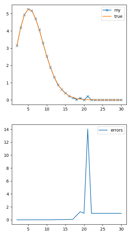
For \(D=2\) we get \(3.14\dots\), which is \(\pi\). That prefactor in the volume goes up till \(D=5\). That’s the number of dimensions in which a sphere is maximally filling. After that, it decreases like crazy.
This code is really good only up to \(D=15\) or so. After that, the sphere is so small that the number of points \(N_{\rm accepted}\) is basically zero and the error made on the predictions is close to 100%.
This is the same information in a plot. The two solutions seem to agree on that scale, but if you look at the errors (bottom plot), that becomes huge.
BTW, I still think it’s weird. What happens if you pour water in an \(N\)-dimensional spherical ball? Can’t fit any water in it. Wait. What’s \(N\)-dimensional water?